Understanding Variational Auto-Encoder
Intro
Variational Auto-Encoder(VAE) is a widely used approach in unsupervised learning for complicated distributions, the application of which includes image generation,representation learning and dimensionality reduction etc. Though often associated with Auto-Encoder in terms of the similarity in the network architecture, VAE’s theoretical foundation and mathematical formulation is quite different. Therefore we are gonna talk about what makes VAE so different and explain how VAE bridges the “variational” method and the “auto-encoder”.
This blog is divided into two parts, with the first one focusing on the statistical concepts and derivation of VAE, while the second more about the practice. PART I will introduce you the problems that VAE is proposed to address, the role played by the “variational” method in the problem solving process, and the connection VAE has with AE. In PART II, we will build our own VAE with pytorch and run the experiment on MNIST dataset.
You are always encouraged to check the original paper, Auto-Encoding Variational Bayes, for further detailed information. A google colab notebook for the experiment and visualization in PART II is also open for exploration.
PART I: Mathematics Behind VAE
PART I is about the mathematical derivation, by which we would make a through explanation about VAE’s model architecture, learning algorithm and contributions.
The Problem Scenario
Let’s consider some dataset $\mathbf{X} = \{ \mathbf{x}^{(i)} \}_{i=1}^N$ consisting of $N$ i.i.d. samples of a random variable $\mathbf{x}$ (either scalar or vector). The data are assumed to be generated by some random process, involving an unobserved random variable $\mathbf{z}$ (i.e. the latent variable).
The generative process has two steps:
- a value $\mathbf{z}^{(i)}$ is generated from some prior distribution $p_{\theta}(\mathbf{z})$,
- a value $\mathbf{x}^{(i)}$ is generated from some conditional distribution $p_{\theta}(\mathbf{x}|\mathbf{z}=\mathbf{z}^{(i)})$ dependent on $\mathbf{z}^{(i)}$,
where the prior $p_{\theta}(\mathbf{z})$ and likelihood $p_{\theta}(\mathbf{x}|\mathbf{z})$ are both parametric distributions of a unknown parameter set $\theta$.
We are interested in solving the following problems related to the given scenario:
- the posterior inference of the latent variable $\mathbf{z}$ given an observed value $\mathbf{x}$ for a choice of parameters $\theta$, i.e. $p_\theta(\mathbf{z}|\mathbf{x})$, which is useful for representation learning.
- the marginal inference of the variable $\mathbf{x}$, i.e. $p(\mathbf{x})$, which is useful in the scenarios where a prior over $\mathbf{x}$ is required.
- the MAP/ML estimation for the parameter set $\theta$, with which one can mimic the above-mentioned generative process and create artificial data.
The Variational Method
This section would introduce you the variational method, which is the key for addressing the three proposed problems. Now let us begin with the posterior inference, i.e. calculating $p_\theta(\mathbf{z}|\mathbf{x}=\mathbf{x}^{(i)})$. We can write down the posterior probability by applying Bayes’s Theorem and probability chain’s rule:
$$
\begin{aligned}
p(\mathbf{z}|\mathbf{x}^{(i)}) & = \frac{p(\mathbf{z},\mathbf{x}^{(i)})}{p(\mathbf{x}^{(i)})} \\
& = \frac{p(\mathbf{x}=\mathbf{x}^{(i)}|\mathbf{z}=\mathbf{z}^{(i)})p(\mathbf{z}=\mathbf{z}^{(i)})}{\int_{\mathbf{z}^{(i)}} p(\mathbf{x}=\mathbf{x}^{(i)}|\mathbf{z}=\mathbf{z}^{(i)})p(\mathbf{z}=\mathbf{z}^{(i)}) d\mathbf{z}^{(i)}} \\
& = \frac{p(\mathbf{x}^{(i)}|\mathbf{z}) p(\mathbf{z})}{\int_{\mathbf{z}} p(\mathbf{x}^{(i)}|\mathbf{z}) p(\mathbf{z}) d\mathbf{z}} & \mathrm{simplify\ the\ notation}
\end{aligned}
$$
Assume we have a choice for $\theta$, thus both the specification of the prior distribution $p_\theta(\mathbf{z})$ and the likelihood $p_\theta(\mathbf{x}^{(i)}|\mathbf{z})$ defined by the generative process are known, and theoretically, the posterior $p_\theta(\mathbf{z}|\mathbf{x}^{(i)})$ can be calculated just by doing the integral $\int_{\mathbf{z}} p_\theta(\mathbf{x}^{(i)}|\mathbf{z}) p(\mathbf{z}) d\mathbf{z}$, which involves enumerating all the possible values the unobservable variable $\mathbf{z}$ may have.
However without any simplifying assumptions on $p_\theta(\mathbf{z}|\mathbf{x}^{(i)})$ or $p_\theta(\mathbf{z})$, the integral is intractable, which means the computation complexity of any approach for evaluating the integral including the enumeration operation is exponential.
Variational methods are designed for such situations and allow us to avoid the intractable integral by transforming the inference problem to a optimization problem. According to the variational methods, a recognition model $q_\phi(\mathbf{z}|\mathbf{x}^{(i)})$ is proposed as an approximation to the true posterior $p_\theta(\mathbf{z}|\mathbf{x}^{(i)})$. By minimizing the KL-divergence between $q_\phi(\mathbf{z}|\mathbf{x}^{(i)})$ and $p_\theta(\mathbf{z}|\mathbf{x}^{(i)})$, we can solve the posterior inference problem. To simplify computation, both the parameters $\phi$ and $\theta$ of the recognition model and the generative model will be jointly optimized here.
$$\phi^*, \theta^* = \mathrm{argmin_{\phi, \theta}} \ KL\big(q_{\phi}(\mathbf{z}|\mathbf{x}^{(i)}) ||p_\theta(\mathbf{z}|\mathbf{x}^{(i)})\big)$$
Parameters ${\phi}$ and $\theta$ would be omitted for simplicity in the following deduction.
$$
\begin{aligned}
KL\big( q(\mathbf{z}|\mathbf{x}^{(i)})|| p(\mathbf{z}|\mathbf{x}^{(i)}) \big) & = \int_\mathbf{z} q(\mathbf{z}|\mathbf{x}^{(i)}) \mathrm{log}\frac{q(\mathbf{z}|\mathbf{x}^{(i)})}{p(\mathbf{z}|\mathbf{x}^{(i)})} d\mathbf{z} & \\
& = \mathbb{E_q}[\mathrm{log} q(\mathbf{z}|\mathbf{x}^{(i)})] - \mathbb{E_q}[\mathrm{log} p(\mathbf{z}|\mathbf{x}^{(i)})] & \mathrm{rewrite\ as\ the\ form\ of\ expectation} \\
& = \mathbb{E_q}[\mathrm{log} q(\mathbf{z}|\mathbf{x}^{(i)})] - \mathbb{E_q}[\mathrm{log} p(\mathbf{x}^{(i)}, \mathbf{z})] + {E_q}[\mathrm{log} p(\mathbf{x}^{(i)})] & p(\mathbf{z}|\mathbf{x}^{(i)}) = \frac{p(\mathbf{x}^{(i)}, \mathbf{z})}{p(\mathbf{x}^{(i)})} \\
& = \mathbb{E_q}[\mathrm{log} q(\mathbf{z}|\mathbf{x}^{(i)})] - \mathbb{E_q}[\mathrm{log} p(\mathbf{x}^{(i)}, \mathbf{z})] + \mathrm{log} p (\mathbf{x}^{(i)}) & p(\mathbf{x}^{(i)}) \mathrm{\ is\ irrelevant\ of\ } q \\
& = -\mathrm{ELBO} + \mathrm{log} p (\mathbf{x}^{(i)})
\end{aligned}
$$
The term $\mathrm{log} p (\mathbf{x})$ is a constant, thus can be ignored during the optimization process. Furthermore, we rewrite the evidence lower bound, ELBO:
$$
\begin{aligned}
\mathrm{ELBO} & = - \mathbb{E_q}[\mathrm{log} q(\mathbf{z}|\mathbf{x}^{(i)})] + \mathbb{E_q}[\mathrm{log} p(\mathbf{x}^{(i)}, \mathbf{z})] \\
& = - \mathbb{E_q}[\mathrm{log} q(\mathbf{z}|\mathbf{x}^{(i)})] - \mathbb{E_q}[\mathrm{log} p(\mathbf{z})] + \mathbb{E_q}[\mathrm{log} p(\mathbf{x}^{(i)}| \mathbf{z})] \\
& = -KL\big(q(\mathbf{z}|\mathbf{x}^{(i)}) ||p(\mathbf{z})\big) + \mathbb{E_q}[\mathrm{log} p(\mathbf{x}^{(i)}| \mathbf{z})]
\end{aligned}
$$
The original optimization problem is by now equivalent to:
$$
\phi^*,\theta^* = \mathrm{argmax_{\phi, \theta}}\ - KL\big(q_{\phi}(\mathbf{z}|\mathbf{x}^{(i)}) ||p_\theta(\mathbf{z})\big) + \mathbb{E_{q_{\phi}(\mathbf{z}|\mathbf{x}^{(i)})}}[\mathrm{log} p_\theta(\mathbf{x}^{(i)}| \mathbf{z})]
$$
The Learning Algorithm
With the help of the variational method, we can get rid of the intractable integral in the posterior inference problem. While the next challenge by now waiting for us is to decide what algorithm is used for the optimization problem. All three problems mentioned in the The Problem Scenario section can be well-settled if this challenge can be properly handled.
Just like other deep learning models, we use the stochastic gradient descent for optimization. The loss function (i.e. the negative ELBO) to minimize is
$$
\mathcal{L}(\phi,\theta, \mathbf{x^{(i)}}) = KL\big(q_{\phi}(\mathbf{z}|\mathbf{x}^{(i)}) ||p_\theta(\mathbf{z})\big) - \frac{1}{L}\sum_{l=1}^L [\mathrm{log} p_\theta(\mathbf{x}^{(i)}| \mathbf{z}^{(i, l)})],
$$
where the expectation term $\mathbb{E_q}[\mathrm{log} p(\mathbf{x}^{(i)}| \mathbf{z})]$ is approximated using Monte Carlo method, i.e. averaging the samples $\mathbf{z}^{(i, l)}$ drawn from $q_{\phi}(\mathbf{z}|\mathbf{x}^{(i)})$. With a differentiable loss function, the full learning algorithm for VAE is as follows:
- get the minibatch consisting of $M$ datapoints;
- compute minibatch loss $\frac{1}{M}\sum_{i=1}^M\mathcal{L}(\phi,\theta, \mathbf{x^{(i)}})$;
- compute gradients $\frac{1}{M}\sum_{i=1}^M \nabla_{\phi, \theta} \mathcal{L}(\phi,\theta, \mathbf{x^{(i)}})$;
- apply gradients to update parameters $\phi, \theta$;
- repeat the first 4 steps util convergence.
In practical, the samples $\mathbf{z}^{(i, l)}$ are not drawn directly from $q_{\phi}(\mathbf{z}|\mathbf{x}^{(i)})$, because $q$ can be a arbitrarily complicated distribution and hard to sample. Therefore, to improve sampling efficiency, we turn to reparameterization trick by setting $\mathbf{z}^{(i, l)} = g_{\phi}(\epsilon^{(i;l)}; \mathbf{x}^{(i)})$, where $g_{\phi}$ can be any neural network which takes $\epsilon^{(i;l)}$ and $\mathbf{x}^{(i)}$ as input and the noise $\epsilon^{(i;l)}$ is sampled from some simple distribution $p(\epsilon)$ (e.g. gaussian).
In addition to the sampling efficiency, another advantage of the reparameterization trick is that it allows better and more overall optimization over $\phi$ and $\theta$. Assume that we directly drew samples from $q_{\phi}(\mathbf{z}|\mathbf{x}^{(i)})$, by doing so, the gradients of the MC estimate term $- \frac{1}{L}\sum_{l=1}^L [\mathrm{log} p_\theta(\mathbf{x}^{(i)}| \mathbf{z}^{(i, l)})]$ would only be back-propagated till the sampling code $\mathbf{z}^{(i, l)}$, the gradients w.r.t $\phi$ would not be computed. Under such circumstance, the parameter $\theta$ can only be optimized by the KL divergence term in the loss, which is not ideal for the learning stability.
VAE vs. AE
This section would make a comparison between VAE and AE to help us have a better understanding of VAE in the perspective of the Auto Encoding Theory.

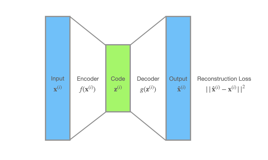
In auto-encoders’ world, a datapoint $\mathbf{x}^{(i)}$ is processed by the encoder $f(\mathbf{x})$ and then a code $\mathbf{z}^{(i)}$ is produced. The decoder $g(\mathbf{z})$ takes the code $\mathbf{z}^{(i)}$ as input and gives us the reconstruction $\hat{\mathbf{x}}^{(i)}$. The reconstruction loss $\mathcal{L}(\mathbf{x}^{(i)})$, is often the squared error, $||\hat{\mathbf{x}}^{(i)} - \mathbf{x}^{(i)}||^2$.

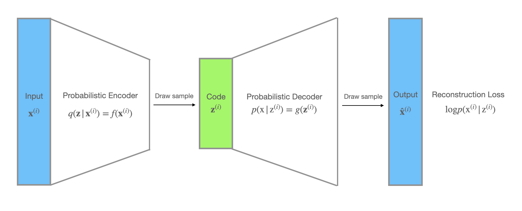
When it comes to VAEs, the unobserved variables $\mathbf{z}$ can be interpreted as the code. In addition, the recognition model $q_{\phi}(\mathbf{z}|\mathbf{x})$ can be treated as a probabilistic encoder, since given a datapoint $\mathbf{x}$ it produces a distribution over the possible values of $\mathbf{z}$, while $p_\theta(\mathbf{x}| \mathbf{z})$ can be seen as a probabilistic decoder, since given a code $\mathbf{z}$, it produces a distribution over the possible corresponding values of $\mathbf{x}$.
The negative log likelihood $-\mathbb{E_{q_{\phi}(\mathbf{z}|\mathbf{x}^{(i)})}}[\mathrm{log} p_\theta(\mathbf{x}^{(i)}| \mathbf{z})] \sim - \frac{1}{L}\sum_{l=1}^L [\mathrm{log} p_\theta(\mathbf{x}^{(i)}| \mathbf{z}^{(i, l)})]$ is used as the reconstruction loss. Besides, there is a KL divergence term in the loss function which acts as a regularizer and enforces the distribution $q_{\phi}(\mathbf{z}|\mathbf{x}^{(i)})$ to stay close to the prior $p_{\theta}(\mathbf{z})$.
Takeaways
To sum up, the following are the takeaways of the first part:
- VAE is proposed to the address three statistical problems, which are respectively the parameter estimation, the posterior inference, and the marginal distribution inference.
- By using variational methods, we can construct a parameter optimization problem whose loss function is Negative ELBO, which can be solved by the reparameterization trick and stochastic gradient descent algorithm.
- The recognition model $q_\phi(\mathbf{z}|\mathbf{x})$ introduced by the variational method, and the pre-defined generative model $p_\theta(\mathbf{x}|\mathbf{z})$ corresponds to the probabilistic encoder and decoder, while the loss function can be interpreted as the combination of the reconstruction loss as well as a regularizer.
PART II: VAE Practical
In this part, for a better understanding, we will present you a case of applying VAE to the MNIST dataset. Besides, we would implement a VAE using Pytorch on our own according to the mathematics in the PART I, and run several experiments.
a VAE for MNIST
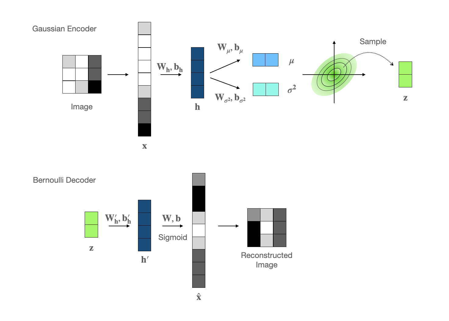
For the MNIST task, the VAE model architecture is constructed as follows:
gaussian encoder
Due to its stable statical property and simplicity in sampling, we choose multi-variate gaussian as the encoder output distribution, where the mean and variance values are modelled by a feedforward network. The parameter set $\phi$ includes $\mathbf{W_h},\mathbf{b_h},\mathbf{W_\mu},\mathbf{b_\mu},\mathbf{W_{\sigma^2}},\mathbf{b_{\sigma^2}}$.$$
\begin{align}
\mathbf{h} & = tanh(\mathbf{W_h}\mathbf{x} + \mathbf{b_h}) \\
\mathbf{\mu} & = \mathbf{W_\mu}\mathbf{h} + \mathbf{b_\mu} \\
\mathbf{\sigma}^2 &= exp(\mathbf{W_{\sigma^2}}\mathbf{h} + \mathbf{b_{\sigma^2}}) \\
q(\mathbf{z}|\mathbf{x}) & = \mathcal{N}(\mathbf{z}; \mathbf{\mu}, \mathbf{\sigma}^2 \mathbf{I})
\end{align}
$$bernoulli decoder
The MNIST data are gray-scale images, of which each pixel can be represented as a float number between 0 and 1, therefore Bernoulli distribution become our first choice for the decoder. The free parameters $\theta$ are $\mathbf{W}_h’,\mathbf{b}_h’,\mathbf{W},\mathbf{b}$.$$
\begin{align}
\mathbf{h’} & = tanh(\mathbf{W_h’}\mathbf{z} + \mathbf{b_h’}) \\
p(\mathbf{x}|\mathbf{z}) & = f_{\sigma}(\mathbf{W}\mathbf{h’} + \mathbf{b}) \\
\end{align}
$$
where $f_{\sigma}$ is the element-wise sigmoid activation function.loss function
For simplicity, we set the prior $p(\mathbf{z})$ as the normal distribution $\mathcal{N}(\mathbf{0}, \mathbf{I})$. The distribution of the probabilistic encoder is $\mathcal{N}(\mathbf{z}; \mathbf{\mu}, \mathbf{\sigma}^2 \mathbf{I})$, where $\mathbf{\mu} \in R^J, \mathbf{\sigma}^2 \in R_+^J$ and $\mu_j, \sigma^2_j$ is the $j$-th component of the mean/var vector respectively. The KL divergence term is:$$
KL\big(q_{\phi}(\mathbf{z}|\mathbf{x}^{(i)}) ||p_\theta(\mathbf{z})\big) = \frac{1}{2} \sum_{j=1}^J(1 + 2\mathrm{log}\sigma_j - \mu_j^2 - \sigma_j^2)
$$As for the expectation term, we set $L=1$ and use the MCMC estimate $\mathrm{log} p(\mathbf{x}^{(i)}| \mathbf{z}^{(i, 1)})$ to take the place of the original expectation term, where the code $\mathbf{z}^{(i, 1)}$ is sampled by the reparameterization trick. Specifically, $\mathbf{z}^{(i, 1)} = \mathbf{\mu} + \mathbf{\sigma} \odot \epsilon$, where the noise $\epsilon \sim \mathcal{N}(\mathbf{0}, \mathbf{I}), \epsilon \in R^J$, and $\mathbf{\mu}, \mathbf{\sigma}^2$ are the mean/var vector in the encoder.
The full loss function (negative ELBO) can be obtained by combing the KL and MCMC estimate terms:
$$
\mathcal{L}(\phi,\theta, \mathbf{x^{(i)}}) = \frac{1}{2} \sum_{j=1}^J(1 + 2\mathrm{log}\sigma_j - \mu_j^2 - \sigma_j^2) - \mathrm{log} p(\mathbf{x}^{(i)}| \mathbf{z}^{(i, 1)}) \\
\mathbf{z}^{(i, 1)} = \mathbf{\mu} + \mathbf{\sigma} \odot \epsilon \\
\epsilon \sim \mathcal{N}(\mathbf{0}, \mathbf{I})
$$

Pytorch Implementation
Here goes the pytorch code for implementing a VAE for the MNIST task.
1 | class GaussianEncoder(torch.nn.Module): |
1 | class BernoulliDecoder(torch.nn.Module): |
Below is the full code for the VAE model that consists of the Gaussian encoder and the Bernoulli decoder. You may refer the github code for more details of training the VAE model.
1 | class VAEModel(torch.nn.Module): |
Experiment on MNIST dataset
As shown below, we evaluated the convergence performance of our VAE on MNIST dataset by comparing testset ELBO values with different dimensionality of the latent variable $\mathbf{z}$. The larger the latent dimensionality is, the higher ELBO value can we achieve and the better the model can learn. However significant overfitting is not observed even when setting dimensionality as 200 (the rightmost panel), due to the regularization effect of the KL divergence.

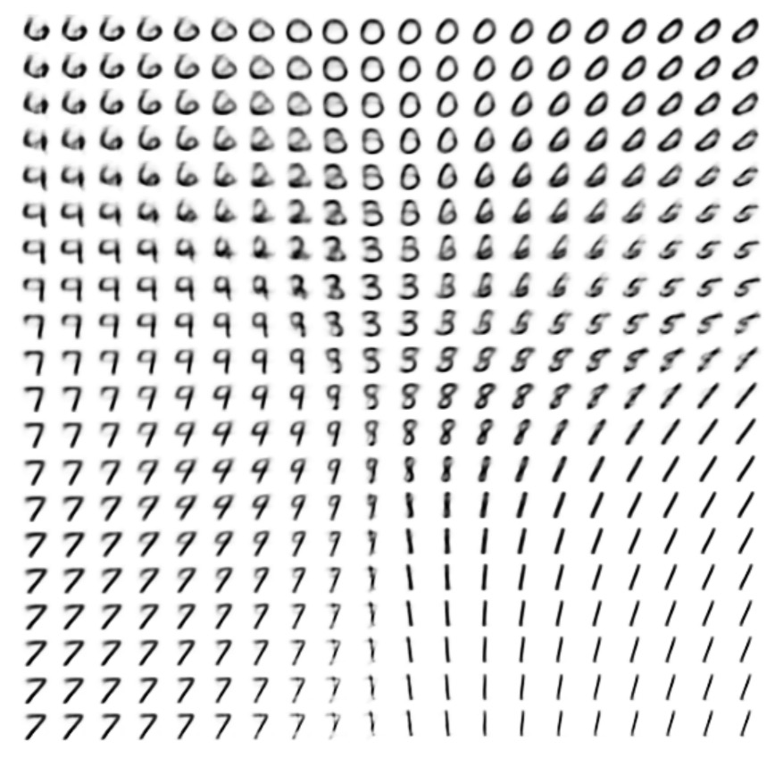
Also, we visualized the 2D manifold learned from the given data.
A google colab notebook is provided here for further exploration.